Time is confusing. Sometimes, it's so confusing that our thinking about it changes... over time. Which makes it triply confusing, or something. In this post, I want to talk about two aspects of temporal data, both common, useful and often misunderstood:
- Homogeneous vs Inhomogeneous
- Temporal vs Bitemporal
Homogeneous Temporal Data
 The first thing to stress is that we're talking about
homogeneous data, because "homogenous" means something completely different.
In a homogeneous, temporal data set, one column will contain a known sequence of discrete time values, and the other columns will contain whatever information is associated with those times.
You would query for an exact match in time, e.g., in SQL
select * where time=3
and expect to find data exactly where you asked for it.
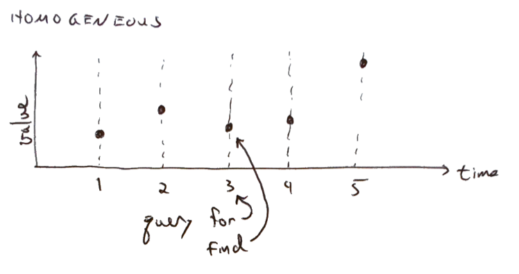 Such a data set might contain a daily closing stock price, or the maximum temperature observed in each
hour of the day -- anything, as long as the time values are discrete and known, and you expect to find
data at every one of them.
Inhomogeneous Temporal Data
By contrast, inhomogeneous temporal data holds observations that occur at arbitrary times. You typically query for information as of a point in time, expecting to get back the most recent observation that isn't after the query time:
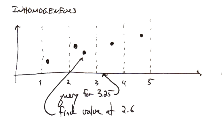
In SQL, the query is a bit awkward
   select * where time <= 3.25
            order by time desc
            limit 1
but would be reasonably efficient in many databases, as long as time was indexed properly.
There's an an O(log N) to find the first acceptable time value, and then we just return it. (Some
databases will pathologically insist on realizing the entire set of previous times, in which case
you'll have to do something cleverer.)
Such a data set might contain posted limit orders for a given stock, or someone's home address indexed by the time they moved into it. The time values are generally not known in advance, and you certainly don't expect to find data at every possible time.
Bitemporal Data
Bitemporal data is inhomogeneous data where we care not just about the time to which the data pertains, but also about the time when we started thinking that did.
True story. Earlier this year, I decided to write down the recent history of my residences:
   Move-in  Address
   20100608 705 Hauser Street, Queens
   20111013 212B Baker Street, London
   20131125 33 Windsor Gardens, London
   20140101 742 Evergreen Terrace, Springfield
Last week, a friend reminded me that I was briefly the Prime Minister of England, so I had to revise the list. Then, last night while I was falling asleep, I suddenly remembered that I had moved in with the Browns on Hallowe'en, and that their address was actually 32. At this point, it seemed like a good idea to record what I had thought and when, if only so I could reconstruct which lies I had told on which credit card applications:
   TT       TV       Address
   20140111 20100608 705 Hauser Street, Queens
   20140111 20111013 212B Baker Street, London
   20140512 20120714 10 Downing Street, London
   20140111 20131125 33 Windsor Gardens, London
   20140512 20131031 32 Windsor Gardens, London
   20140111 20140101 742 Evergreen Terrace, Springfield
In the spirit of academic rigor, I labeled my columns with the standard convention of TV for
the time to which the value pertains and TT for the transaction time when it was
entered into the ledger.
Purely functional queries
Enough about me; let's switch to some fictional data. The TV-axis below denotes the time at which a measurement was taken. The value of the measurement is recorded as vertical height, and the time it was recorded is on the TT-axis.
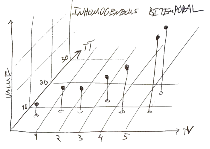
As of TT=10, we knew about points at TV=0.6, 1.5, 2.5, 4.4 and 5.6; at TT=12, we learned about a new measurement at TV=3.5; at TT=17, we revised the measurement at TV=5.6 to a slightly higher value.
Now, imagine a query for TV=4, TT=10. It's not particularly graceful to cram this into SQL, but if we did, the query would be something like:
  select * where TV<=4 and TT<=10
           order by TV desc, TT desc
           limit 1
Note that this won't always be efficient, for reasons we'll discuss below. Graphically, the blue arrows below start at the point of the query and end at the resolved value for queries as of (TV=4, TT=10) and (TV=6, TT=10):
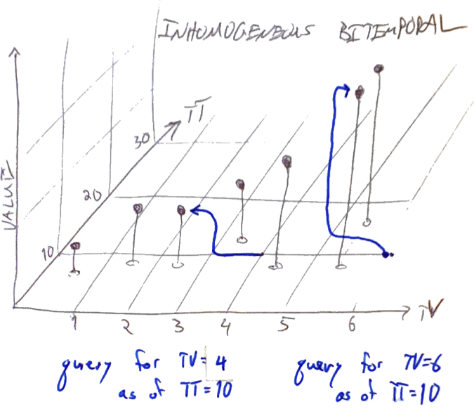
If we executed the same queries but with TT=20, the resolutions would be different, as shown in red:
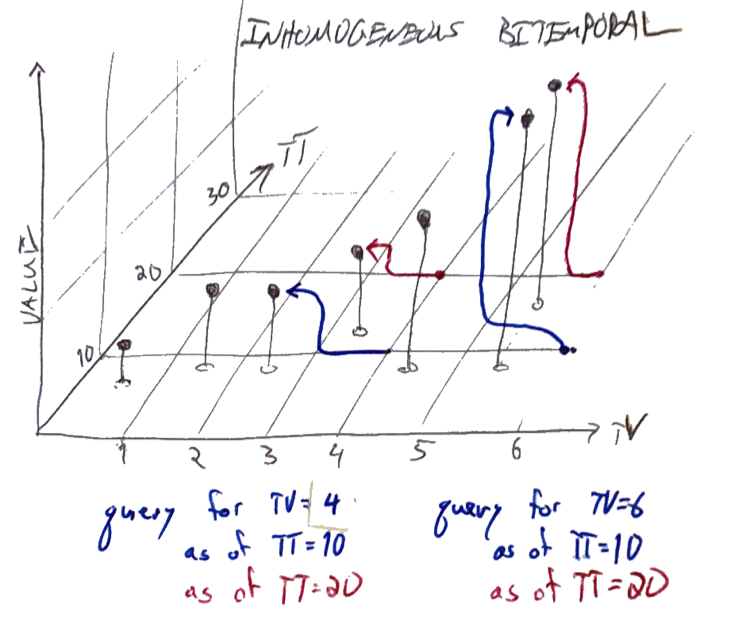
Now, the most recent value visible as of TV=4 is from 3.5 rather than 2.5; similarly, the query at TV=6 continues to see the point from 5.6, but now it has been "overwritten" to a different value.
Of course, nothing was really overwritten: if we repeated the query at TT=10, we'd still get back the blue results. If we can promise that
- transactions occur at strictly increasing TTs and
- we never query for TT in the future beyond the next transaction TT
which is most easily achieved by
- using the physical clock time for TT in transactions and
- never querying for TT in the future,
then a query for any given (TT,TV) pair will always return the same result, and querying is a purely functional operation.
Asymmetry
Here's a 2D view from below of a similar dataset: TV is on the x-axis; TT is on the y-axis, and we're recording the color of a lamp, which can be green, blue, red or splotchy purplish. Here, the region below the diagonal line is forbidden by causality, since we can't possibly record something before we observe it.
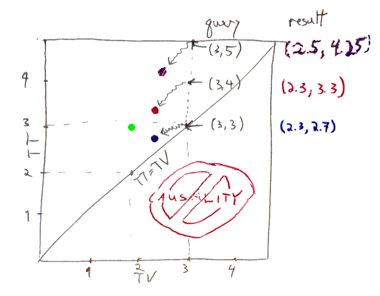
As of TT=3, there are two observations recorded, green at (TV=1.9, TT=2.9) and blue at (TV=2.3, TT=2.7) A query for (TV=3, TT=3) will find the blue point at (TV=2.3, TT=2.7).
Why not green at (1.9, 2.9), which is further from TV but closer to TT? Because TT and TV are not precisely symmetric. We are asking the question, "at TT=3.0, what did we think the color of the lamp was at TV=3.0?". The alternate question, "what is the most recently recorded information as of TT=3.0 concerning the lamp's status at some time at or before TV=3.0?" is poseable, but not usually what we want.
 At 3.3, we we spoke to a passing
samurai
who told us that, notwithstanding
previous
reports,
the lamp was actually red.
Finally, at 4.25, a local
woodcutter
suggested that we split (get it?) the difference and call it splotchy purple.
Based on this revision history, queries for TV=3 as of TT=3, 4 and 5, respectively, would return blue, red and purple.
Efficiency
As noted above, a single-sided SQL range query for both TV and TT is likely to be quite wasteful. Typically, the optimizer will
- Pick one of the two temporal columns, say TV for concreteness, but it could be either.
- Do an O(log N) search to find the most recent acceptable TV value.
- Scan down through TV, assembling a realization of all M rows matching the TT and TV constraints, taking O(N) time and O(M) space.
- Sort them by TT, taking O(M log M) time.
- Take the first and discard the rest of the realization.
This is unacceptable for all but the tiniest data sets.
For many use cases, we can do better. Commonly, we can assume:
- TT >= TV - i.e. we are storing observations, not predictions. (As in the examples above.)
- Revisions are infrequent.
Typically, then, every datapoint will have just one observation, with TT slightly later than its TV This can be then be nicely represented in a multi-column index, which essentially stores a sorted structure of concatenations of TV and TT. For the address example, it would look like
TV:TT             Address
20100608:20140111 705 Hauser Street, Queens
20111013:20140111 212B Baker Street, London
20120714:20140512 10 Downing Street, London
20131125:20140111 33 Windsor Gardens, London
20131031:20140512 32 Windsor Gardens, London
20140101:20140111 742 Evergreen Terrace, Springfield
If I were looking, say, for what I thought on Valentines day 2014 that my address had been on Christmas of 2013, the query would
- Perform O(ln N) search for the last TV:TT that is alphabetically less than or equal to "20131225:20140214".
- Find "20131031:20140512", which violates the TT constraint.
- Scan backwards until TT <= 20140214.
- Hit "20131125:20140111" immediately.
- Bother Paddington's neighbor.
This index and query would work even without the assumptions above, but it might be more costly. E.g.
- If there were a huge number of revisions, we would have to scan through them all.
- If we queried for a TT very much earlier than the desired TV, we might well scan backwards through the entire data set before concluding that there was no such entry.
Bitemporality with Datomic
Datomic is a commercial database, invented by Rich Hickey and sold by Cognitect. It has many desirable features, but for our purposes, three are important:
- The database is a persistent data structure.
- It has built-in TT-style temporality.
- It has a nice clojure API.
So there is a distinction between a connection
(def conn (d/connect "datomic:free://localhost:4334/bitemp"))
and a database.
(def db (d/db conn))
The latter is a private, persistent, immutable object, and nothing anybody else does, now or in
the future, can affect the results of queries we make against it, as long as its in scope. Of course,
if we call d/db sometime later, its return value will "contains" any transactions executed
in the interim. We can, if we want, be precise about exactly what interim means:
(def db (d/as-of (d/db conn) tx-time))
All dbs thus obtained with a particular tx-time will contain exactly the same data.
By implication, anything placed into Datomic is immutable. An existent value can't change, but a new
one can be added.
For consistency, transaction time is strictly increasing across the entire system; it is exactly what we're looking for in a TT. TV, however, we'll have to roll ourselves. As a concrete example, let's implement a simple bitemporal store. It could hold things like stock prices for random tickers at random times of the day, colors of lamps, addresses - anything observed at discrete times, then recorded and possibly revised later. The code, such as it is, is on github; what I show here will be abbreviated for clarity.
Stripped of some boilerplate (i.e. this won't actually run), the schema defines four attributes:
    [{:db/ident :bitemp/k
      :db/valueType :db.type/string
      :db/doc "Non-temporal part of the key"}

     {:db/ident :bitemp/tv
     :db/valueType :db.type/instant
     :db/doc "Time for which data is relevant"
     :db/index true}

     {:db/ident :bitemp/index
      :db/valueType :db.type/string
      :db/doc "This is the mysterious and exciting part."
      :db/unique :db.unique/identity}

     {:db/ident :bitemp/value
      :db/valueType :db.type/string
      :db/doc "The value"}
     ]
The k field is the non-temporal identifier of whatever we're measuring. It could be a stock
ticker, the name of the person whose address we're tracking, the location of colorful lamp, etc.
We explicitly keep tv; its instant type is basically a java data, which is basically
a number of milliseconds since the great epoch. Datomic will take care of TT.
Per the comments, :bitemp/index attribute is mysterious and exciting, so ignore what it does for the
moment.
We can insert a value with something like:
(defn insert-tx [k tv value]
  (let [tv  (jd tv)
        idx (idxid k tv)]
    {:db/id (d/tempid :bitemp)
                          :bitemp/index idx
                          :bitemp/k k
                          :bitemp/tv tv
                          :bitemp/value value}))
(defn insert-value [conn k tv value]
  (-> @(d/transact conn [(insert-tx k tv value)])
      :tx-data first  .v))
The return value will be the transaction time.
Magic, part I
If we knew the exact TV we were looking for, we could query straightforwardly. In Datalog:
(defn query-exact [conn k tv tt]
  (d/q '[:find ?v :in $ ?k ?tv :where [?e :bitemp/k ?k]
                                      [?e :bitemp/tv ?tv]
                                      [?e :bitemp/v ?v]]
       (d/as-of (d/db conn) tt) k tv))
This finds a database as of tt, looks in it for an entity (as inserted above) with a
specific k and tv, binds its ``vto?v``` and returns it.
Generally, we don't know exactly what TV to look for, which is where index comes in.
Datomic has an index-range function, which, for an indexed attribute, returns a lazy sequence
starting at the first entry greater than or equal to a specified value and increasing.
We want to devise entries
for this index such that this function will quickly locate that an exact match for k and
the first tv less than or equal to a target. The comparison value of our entries must
therefore decrease with increasing tv. We construct the field as follows:
(defn k-hash [k] (digest/md5 k))
(defn long->str [l]
  (let [li (- 100000000000000 l)]
    (apply str (map #(->> % (bit-shift-right li) (bit-and 0xFF) char) [56 48 40 32 24 16 8 0]))))
(defn t-format [t] (-> t .getTime long->str))
(def idx-sep "-")
(defn idxid [k tv] (str (k-hash k) idx-sep (t-format tv)))
The index will look like "e757fd4fedc4fe825bb81b1b466a0947-^@^@(#&%($"
Before the hyphen, we have
the md5 hash of the non-temporal part of the key. After the hyphen, we have TV in milliseconds,
subtracted from 10^14, and crammed into 8 characters.
For an exact k and a target tv, I
can construct the string and take the head of the sequence returned by index-range:
(defn get-at [conn k tv tt]
  (let [tvf (t-format tv)
        kh  (k-hash k)
        idx (str kh idx-sep tvf)
        db  (-> conn db (d/as-of (first  tt)))
        e   (some-> (d/index-range db :bitemp/index idx nil)
                    seq first .v)]
    (or  (and e (.startsWith es kh)
              (first (q '[:find ?tv ?v
                          :in $ ?i ?k
                          :where
                          [?e :bitemp/index ?i]
                          [?e :bitemp/k     ?k]
                          [?e :bitemp/value ?v]
                          [?e :bitemp/tv   ?tv]]
                        db e k)))
         nil)))
The (or (and e (.startsWith es kh)... business takes care of the possibilities that
index-range returned false, or that there were no appropriate tvs, so it fell through
to the next k.
When we call get-at, the TT part of the query is handled by Datomic's as-of, while the
TV part uses our fancy composite index.
Magic, part II (or the lack thereof)
It's all very well and good to say that Datomic is "handling" the TT query, but how exactly
is it doing that? Datomic's persistent data structures are clever, but under the covers they must be
susceptible to the complexities discussed above in the Efficiency section.
Datomic being closed source, it's hard to find out exactly how it executes queries, but some
information has been gleaned from
forums and lectures. It seems that
   To answer as-of query for moment T, current, in-memory and
   history parts get merged, and then all data with timestamp after
   moment T is ignored. Note that as-of queries do not require
   older versions of current index, they use most recent current
   index and filter it by time, deducing the previous view of the
   database.
So we're implicitly making the assumption proposed above, of infrequent revisions. If revisions for the same query parameters are rampant, then Datomic will scan over the set of all versions and "filter it by time", which will, as in the SQL case, be dreadful.
To test this implementation realistically, we'll want to insert a lot of entries, and to do so in reasonable batch sizes. A single transaction can of course encompass multiple operations:
(defn insert-values [conn k-tv-values]
  "Insert multiple values at [[k1 tv1 v1] [k2 tv2 v2] ...] and return the transaction single time"
  (-> @(d/transact conn (map (partial apply insert-tx) k-tv-values))
      :tx-data first  .v))
Since I can't think of any more funny addresses, the test will involve random data.
In a single transaction, we'll insert things like nKeys different keys, of the form Thing${kKey};
we'll do this over nTv explicitly different times; and we'll repeat the exercise nTt times,
implicitly picking up increasing transaction times, which we then return. The values will be of
the form Thing${kKey}v${jTv}t${iTt} so we can easily verify later if they're correct.
(defn insert-lots [conn nKeys nTv nTt]
  "Insert lots of stuff.  nKeys unique keys, nTv tv's, nTt nt's in batches of nKeys.
Returns a list of nTt transaction times suitable for passing into query-lots."
  (for [iTt (range nTt)]
          (last (for [jTv (range nTv)]
                    (do  (insert-values conn
                                      (for [k (range nKeys)]
                                          (let [k  (str "Thing" k)
                                             tv (jd (* 10  jTv))
                                             v  (str k "v" jTv "t" iTv)]
                                             [k tv v]))))))))
Note that we've made explicit choices about how easy to make this for Datomic.
Remember that the index is going to be stored in an order that is first increasing in kKey
and then decreasing in jTv. For every (kKey,jTv), there will be a block of differing
transaction times. So our insertions are in a raster pattern:
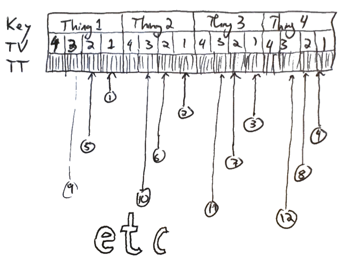
Depending on our planned access patterns, we might want to restructure our index key someday, so that temporally proximate insertions are spatially proximate as well. For example, if we were storing stock prices that tended to arrive in increasing TV, we might put that part of the key first. Our decision will reflect both our access patterns (which we may be able to know in advance) and Datomic's caching strategy (which is a little less clear and, unfortunately, not directly observable).
For batches of 20 or so keys, on the free, local storage variant of Datomic, insertions stabilize at around
750-1000 microseconds. Random reads (note the assertion that we're finding the values we looked for)
(defn query-lots [conn nKeys nTv tts n]
  (let [tts (vec tts)
        nTt  (count tts)]
    (dotimes [_ n]
      (let [i  (rand-int nTt)
            tt (get tts i)
            j  (rand-int nTv)
            tv (jd  (* 10 j))
            k  (str "Thing" (rand-int nKeys))
            v  (second (get-at conn k tv tt))
            ve (str k "v" j "t" i) ]
        (assert (= v ve))
        ))))
stabilize at around 500-750 microseconds, even for data volumes in excess of JVM heap size.
In conclusion, Datomic is a very promising option for storing inhomogeneous bitemporal data, but we
must always think carefully about how are access will actually be implemented, to avoid cache thrashing.
The presentation of the database as a persistent data structure, with scrolling access to previous states,
naturally captures the TT dimension, while TV needs to be implemented schematically; the
assymetrical relationship between the two times means we can't do it the other way around.
Comments
comments powered by Disqus